3. Define Case Settings#
This page will discuss the various settings that can be toggled in a Resolve run.
Most settings on the “Resolve Settings” tab are formula-linked to pre-populated settings on the “Case List” tab.
You can update these settings by adding columns to the “Case List” tab.
2023 CPUC IRP
CPUC IRP stakeholders will find case settings for all the cases posted on the CPUC website pre-populated on the “Case List” tab.
Case Settings#
Input Scenarios#
See Scenario tagging functionality for discussion about how to input scenario tagged data for components & linkages.
As discussed in resolve.common.component.Component.from_csv(), input scenario tags are prioritized
based on the order of scenarios in the Resolve case. Scenarios listed toward the bottom of the scenario list are higher priority
and more likely to override other data if data is tagged with a “lower priority” scenario tag. In the screenshot below, for example,
data tagged with the base tag will the lowest priority, since it is the first tag in the scenario list. For any of the
subsequent scenario tags (e.g., 2021_PSP_22_23_TPP_ITC_ext), to the extent that there is data that is tagged with the higher
priority scenario tag, that higher priority data will override any base-tagged data.
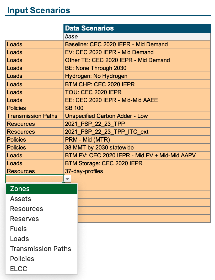
On the Resolve Settings tab, users will find an orange dropdown inputs menu to help ensure that input scenarios selected
are based on scenario tags that already are defined on the respective component & linkage attribute tabs.
In the first column, select the sheet on which to look up available scenario tags. Then, in the second column, the dropdown input
should only present scenario tags that are already defined on the respective sheet of the Scenario Too.
Representative Period Settings#
Toggle between pre-defined sets of sampled days saved in the Scenario Tool. See {ref}`timeseries-clustering for instructions on how to create new sampled days.
Financial & Temporal Settings#
The model will now endogenously calculate the annual discount factors to use for each modeled year based on four pieces of information:
Cost dollar year: The dollar year that costs are input in & should be reported out in. In general,
Resolveis designed to be in real dollars for a specific dollar year.Modeled years: Which modeled years to include in the
Resolvecase.End effect years: The number of years to extrapolate out the last modeled year. In other words, considering 20 years of end effects after 2045 would mean that the last model year’s annual discount factor would represent the discounted cost of 2045-2064, assuming that the 2045 costs are representative of a steady-state future for all end effect years.
Annual discount rate: Real discount rate in each year
Inter-period dynamics: Include additional chronological information to allow
Resolveto shift energy between days across the modeled weather years.
Solver Settings#
For now, users must follow the pattern of solver.[solver name].[solver option].[data type] when setting the solver settings.
For example, users wanting to set Gurobi’s Method setting
would need to enter solver.gurobi.Method.int and the corresponding value.
Custom Constraints#
Custom constraints allow users to customize the functionality of Resolve by adding additional constraints
without needing to change the code. These are defined on the “Custom Constraints” tab and saved to
./data/settings/resolve/[case name]/custom_constraints/
2023 CPUC IRP
For the CPUC IRP, custom constraints are used for various custom functionality:
Resource deliverability (i.e., CAISO FCDS/EO designation) and accompanying CAISO transmission upgrades
Connecting disaggregated build variables to aggregate operational resources (which allows
Resolveto make granular investment decisions while reducing the model size needed to represent operations.Group-level constraints (e.g., “Resolve must build 15 GW of offshore wind by 2045” but can select amongst the 4 candidate OSW resources.)
To create custom constraints:
Create a “Custom Constraint Group” name of your choosing. These groups are toggled on/off in the active case settings together, so group custom constraints accordingly.
Within each custom constraint group,
Timeseries Clustering#
Advanced Topic
Users who want to create a new set of sampled days can do so using the included Jupyter notebook in ./notebooks/cluster.py.
This is a Jupytext file. Note that to run the timeseries clustering, you first must save a case and all
relevant system & component data (as described in saving-inputs).
To open this notebook:
Open a Command Prompt or Terminal and navigate to the
./notebookssubfolderActivate the
resolve-envenvironment usingconda activate resolve-envOpen the notebook using the following commands, which will launch a new tab in your web browser:
jupytext-config set-default-viewer
jupyter lab cluster.py
This will launch a window in your web browser that looks something like this:
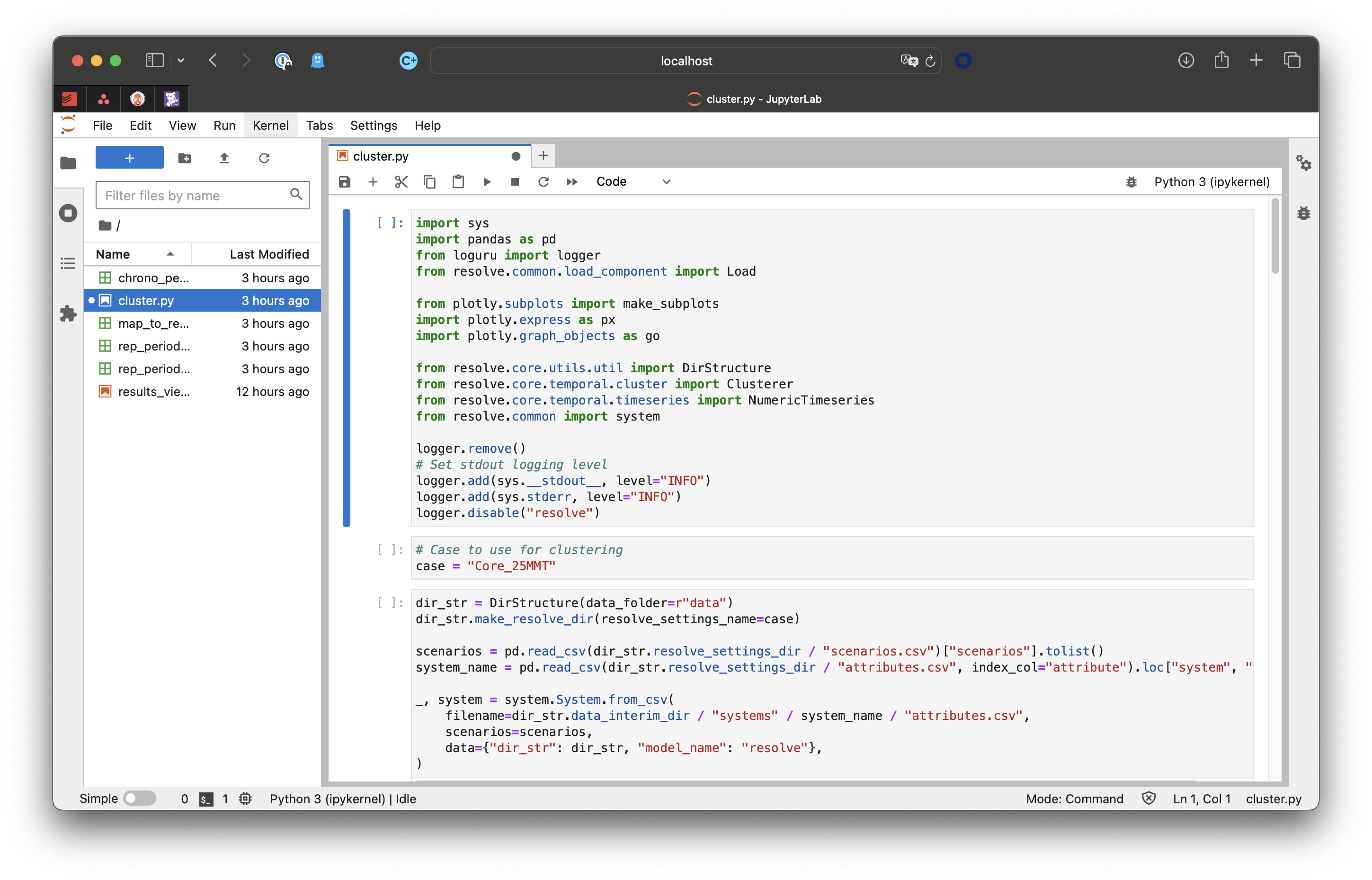
In the second “cell”, change the case name from “Core_25MMT” to the case you want to use. The notebook will then load the case and its corresponding system data to start the timeseries sampling process.
Run the cells (using the button or by using
Shift + Enterkeyboard shortcut). (For Jupyter notebook basics, users can start here).If the notebook runs successfully, a CSV file will be created in the
./notebooksfolder calledmap_to_rep_periods.csv. Paste the data in that CSV into the “Rep Periods” tab of the Scenario Tool (insert columns in the yellow input table areas as-needed).Toggle between different timeseries samples by updating your case settings on the “Case List” tab.