RESOLVE Scenario Tool

The Resolve Scenario Tool is a user-centric model interface, designed to link data, inputs, assumptions, and constraints with the Resolve code. The primary step in being able to make that linkage is making sure that xlwings is correctly set-up

Configuring xlwings

![Overall add a figure for describing the flow of inputs into ST from

1. GEnlist

2. RC&B

3. RP&T co-ordinate w ANgineh]

![Additionally we need to add a Data-catalog - table where the data sources are outlined Eg for load we refer to IEPR… To be decided We can add it to the ST but in the doc we can refer back to it]

We have seen that running resolve requires interfacing with both excel as well as python based code. xlwings is a tool that helps in interfacing excel and python and something that is very necessary for the model to run smoothly

More standalone information on xlwings can be found here:

For our purposes we will focus on installing xlwings and making it work with the Resolve Scenario Tool excel workbook

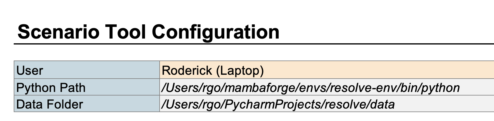
On the Scenario Tool’s Cover & Configuration tab, you will need to tell the Scenario Tool how to find your resolve-env Python path and the data folder where you want to save inputs.

Windows Excel

Configure Python Path:

1. Open Command Prompt or PowerShell and activate the environment with the command conda activate resolve-env

2. Type the command where python to see where the resolve-env version of Python is stored. This should look like: C:\Users\[username]\Anaconda3\envs\resolve-env\python.exe. Paste this path into the Python Path cell.

Warning

Make sure to use a backslash \ (and not a forward slash /) on Windows for the Python path.

Configure Data Folder Path:

By default, this folder is called data and located in the project folder next to the scr folder. For completeness, type the full path to the data folder, may look something like ~/.../resolve/data

macOS Excel

Configure Python Path:

1. Open Terminal and activate the environment with the command conda activate resolve-env

2. First time setup only Run the command xlwings runpython install. You should see a prompt from macOS asking you for permission for Terminal to automate Excel. You must allow this.

3. Type the command which python to see where the resolve-env version of Python is stored. This should look like: /Users/[username]/anaconda3/envs/resolve-env/bin/python. Paste this path into the Python Path cell.

Warning

Make sure to use a forward slash / (and not a backslash \) on macOS for the Python path.

Configure Data Folder Path:

By default, this folder is called data and located in the project folder next to the src folder. For completeness, type the full path to the data folder, may look something like ~/.../resolve/data

---

Structure & Tabs of the Scenario Tool

Scenario Tool Tab	Short Description
Cover & Configuration	Key starting point, takes input for Python & Folder Path as defined by the user
Case List	A tab where users can look at existing case designs, make new cases and record them
RESOLVE Settings	Primary place to save input data and case settings, includes Macros for running cases (More detail on this tab below)
Temporal Settings & Rep Periods	RESOLVE uses representative days o run the simulatuion, additional details on the same can be found on these tabs
System	A tab to define and create new systems that encapsulate all sectors of the electric systems
Loads	Defines different load components and values for the system
Transmission Paths	Defines Tx paths, forward and reverse ratings as well as hurdle rates

The Scenario Tool has a plethora of other information and tabs that all flow into the model. Not all of these tabs are defined in detail in the documentation, however some of the tabs are self-explanatory.

For eg: Different resource types have their own tabs - taking variable resources as an example, the Variable tab lists all the variable resources in the CAISO system, along with what zone they are in, what are the operating characteristics of that resource as well as whether or not there is potential to build additional capacity of that resource.

Additional comprehensive information on some of these inputs and assumptions present in the Scenario Tool can be found in the Inputs & Assumptions document released by the CPUC.

For users planning on comprehensively using the Model, a thorough reading of the I&A document is recommended.

Saving Input Data & Case Settings

Users who want to run pre-existing cases can save all necessary inputs from the “Resolve Settings” tab of the Scenario Tool.

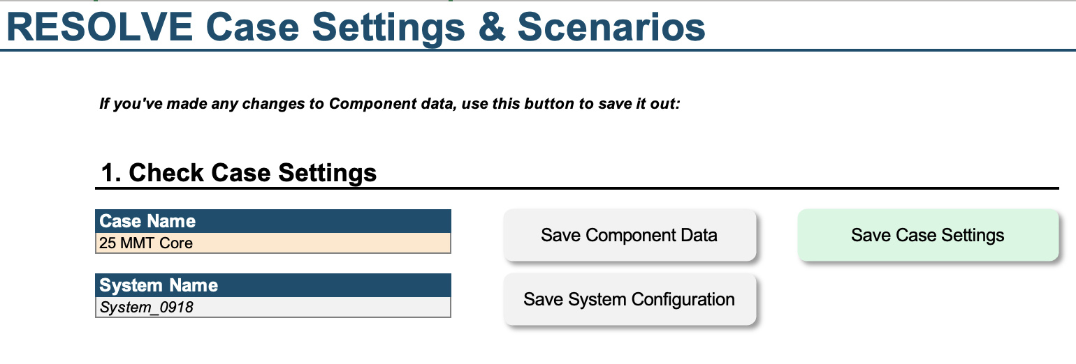
1. Save the Component input data (e.g., resource heat rates, etc.) using the “Save Component Data” button

2. Save the System configuration (i.e., the combination of loads, resources, etc. to model) using the “Save System Configuration” button

3. Save a single case (e.g., years to model, scenarios, etc.) by selecting a case name from the “Case Name” dropdown and pressing the “Save Case Settings” button

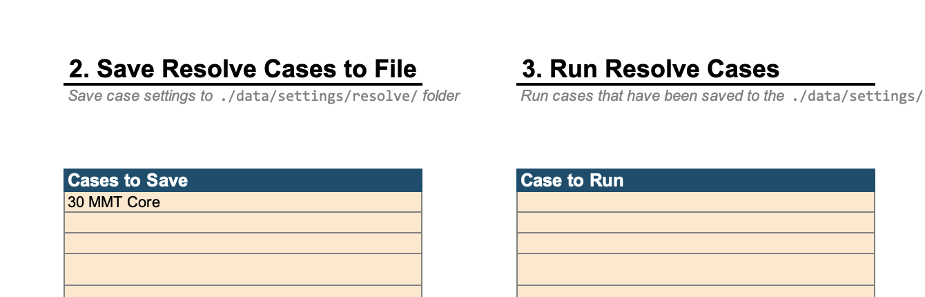
   • To the right side of the “Resolve Settings” tab, you can also save multiple cases out of the Scenario Tool:

---

For users who want to update or create new inputs data, systems, and cases, the subsequent pages discuss how to update data in the Scenario Tool in more detail.

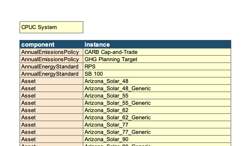
1. Component Data

Components are the fundamental building block of what Resolve models. All Components have attributes that can be set via the Scenario Tool.

Class	Description
AnnualEmissionsPolicy	Annual emissions accounting that can encompass generation & importing transmission paths.
AnnualEnergyStandard	Renewable Portfolio Standard (RPS) or Clean Energy Standard (CES)-type policies.
Asset	Any physical asset where we want to track & optimize investment costs.
CandidateFuel	A fuel that can be used by generators (or created if using electrolytic fuel production)
ELCCSurface	ELCC surface inputs
Load	A load component consisting of an hourly profile and an annual energy and/or peak forecast.
PlanningReserveMargin	A Planning Reserve Margin (PRM) reliability accounting constraint, interacts with ELCCSurface.
Reserve	Operating reserves, such as spin, regulation, load following.
Resource	An Asset used for electric sector operations (e.g., thermal generator, battery, variable resource).
TXPath	Resolve uses a “transportation” (“pipe-and-bubble”) model for transmission flows between zones.
Zone	A location, constrained by transmission, where loads & resources are located.

Scenario tagging functionality

See Input Scenarios for discussion about how to determine which scenario tagged data is used in a specific model run.

On most of the component & linkage attributes tabs, you will find a Scenario column. In the Scenario Tool, a single instance of a component can have multiple line entries in the corresponding data table as long as each line is tagged with a different scenario tag, as shown in the below screenshot.

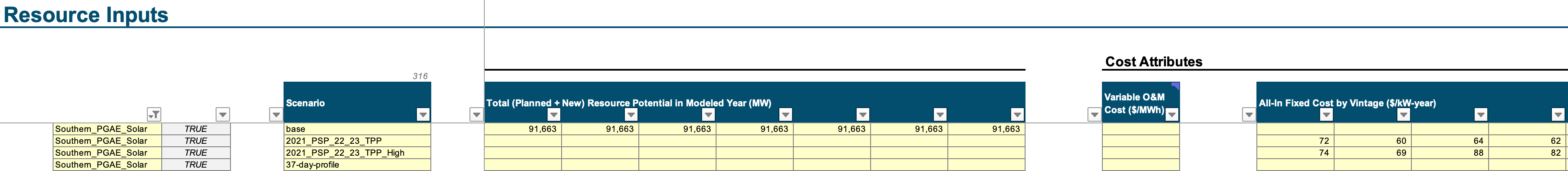
Scenario tags can be populated sparsely; in other words, every line entry for the same resource does not have to be fully populated across all columns in the data tables. In the example screenshot above, this is demonstrated by the base scenario tag having data for “Total (Planned + New) Resource Potential in Modeled Year (MW)” and no data for “All-In Fixed Cost by Vintage ($/kW-year)”, whereas the scenario tags 2021_PSP_22_23_TPP and 2021_PSP_22_23_TPP_High are the reverse.

The Scenario Tool will automatically create CSVs for all the data entered into the Scenario Tool. These CSVs have a four-column, “long” orientation.

timestamp	attribute	value	scenario (optional)
[None or timestamp (hour beginning)]	[attribute name]	[value]	[scenario name]
…	…	…	…

Timeseries Data

Hourly timeseries data is now stored in separate CSV files under the ./data/profiles/ subfolder to keep the Scenario Tool spreadsheet filesize manageable. These CSVs must have the following format:

timestamp	value
[timestamp (hour beginning)]	[attribute value]
…	…

On the Scenario Tool, you’ll see certain data attributes have filepaths as their input, which point the code to the relevant CSV file.

2. Configure a System

The “System” tab defines the energy system being modeled, which is composed of a list of various modeling components (loads, resource, policies, etc.). This tab will have any pre-populated system configurations in the yellow table(s) to the right of the tab, and different systems are linked to the active case on the “Resolve Settings” tab.

If users add any new modeling components (e.g., load components with new names, resources with new names), they will need to make sure that these new components are added to either an existing or new system configuration by updating the system list.

3. Define Case Settings

This page will discuss the various settings that can be toggled in a Resolve run. Most settings on the “Resolve Settings” tab are formula-linked to pre-populated settings on the “Case List” tab. You can update these settings by adding columns to the “Case List” tab.

2023 CPUC IRP

CPUC IRP stakeholders will find case settings for all the cases posted on the CPUC website pre-populated on the “Case List” tab.

Case Settings

Input Scenarios

See Scenario tagging functionality for discussion about how to input scenario tagged data for components & linkages.

As discussed in resolve.common.component.Component.from_csv(), input scenario tags are prioritized based on the order of scenarios in the Resolve case. Scenarios listed toward the bottom of the scenario list are higher priority and more likely to override other data if data is tagged with a “lower priority” scenario tag. In the screenshot below, for example, data tagged with the base tag will the lowest priority, since it is the first tag in the scenario list. For any of the subsequent scenario tags (e.g., 2021_PSP_22_23_TPP_ITC_ext), to the extent that there is data that is tagged with the higher priority scenario tag, that higher priority data will override any base-tagged data.

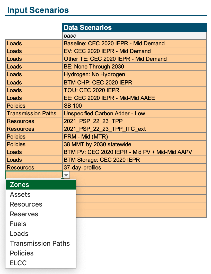
On the Resolve Settings tab, users will find an orange dropdown inputs menu to help ensure that input scenarios selected are based on scenario tags that already are defined on the respective component & linkage attribute tabs. In the first column, select the sheet on which to look up available scenario tags. Then, in the second column, the dropdown input should only present scenario tags that are already defined on the respective sheet of the Scenario Too.

Representative Period Settings

Toggle between pre-defined sets of sampled days saved in the Scenario Tool. See {ref}`timeseries-clustering for instructions on how to create new sampled days.

Financial & Temporal Settings

The model will now endogenously calculate the annual discount factors to use for each modeled year based on four pieces of information:

1. Cost dollar year: The dollar year that costs are input in & should be reported out in. In general, Resolve is designed to be in real dollars for a specific dollar year.

2. Modeled years: Which modeled years to include in the Resolve case.

3. End effect years: The number of years to extrapolate out the last modeled year. In other words, considering 20 years of end effects after 2045 would mean that the last model year’s annual discount factor would represent the discounted cost of 2045-2064, assuming that the 2045 costs are representative of a steady-state future for all end effect years.

4. Annual discount rate: Real discount rate in each year

5. Inter-period dynamics: Include additional chronological information to allow Resolve to shift energy between days across the modeled weather years.

Solver Settings

For now, users must follow the pattern of solver.[solver name].[solver option].[data type] when setting the solver settings. For example, users wanting to set Gurobi’s Method setting would need to enter solver.gurobi.Method.int and the corresponding value.

Custom Constraints

Custom constraints allow users to customize the functionality of Resolve by adding additional constraints without needing to change the code. These are defined on the “Custom Constraints” tab and saved to ./data/settings/resolve/[case name]/custom_constraints/

2023 CPUC IRP

For the CPUC IRP, custom constraints are used for various custom functionality:

• Resource deliverability (i.e., CAISO FCDS/EO designation) and accompanying CAISO transmission upgrades

• Connecting disaggregated build variables to aggregate operational resources (which allows Resolve to make granular investment decisions while reducing the model size needed to represent operations.

• Group-level constraints (e.g., “Resolve must build 15 GW of offshore wind by 2045” but can select amongst the 4 candidate OSW resources.)

To create custom constraints:

1. Create a “Custom Constraint Group” name of your choosing. These groups are toggled on/off in the active case settings together, so group custom constraints accordingly.

2. Within each custom constraint group, define…

3. To be able to include a set of constraints the user needs to add the name of the custom constraint group to the case settings tab

Timeseries Clustering

Advanced Topic

Users who want to create a new set of sampled days can do so using the included Jupyter notebook in ./notebooks/cluster.py. This is a Jupytext file. Note that to run the timeseries clustering, you first must save a case and all relevant system & component data (as described in Saving Input Data & Case Settings).

To open this notebook:

1. Open a Command Prompt or Terminal and navigate to the ./notebooks subfolder

2. Activate the resolve-env environment using conda activate resolve-env

3. Open the notebook using the following commands, which will launch a new tab in your web browser:

jupytext-config set-default-viewer
jupyter lab cluster.py

This will launch a window in your web browser that looks something like this:

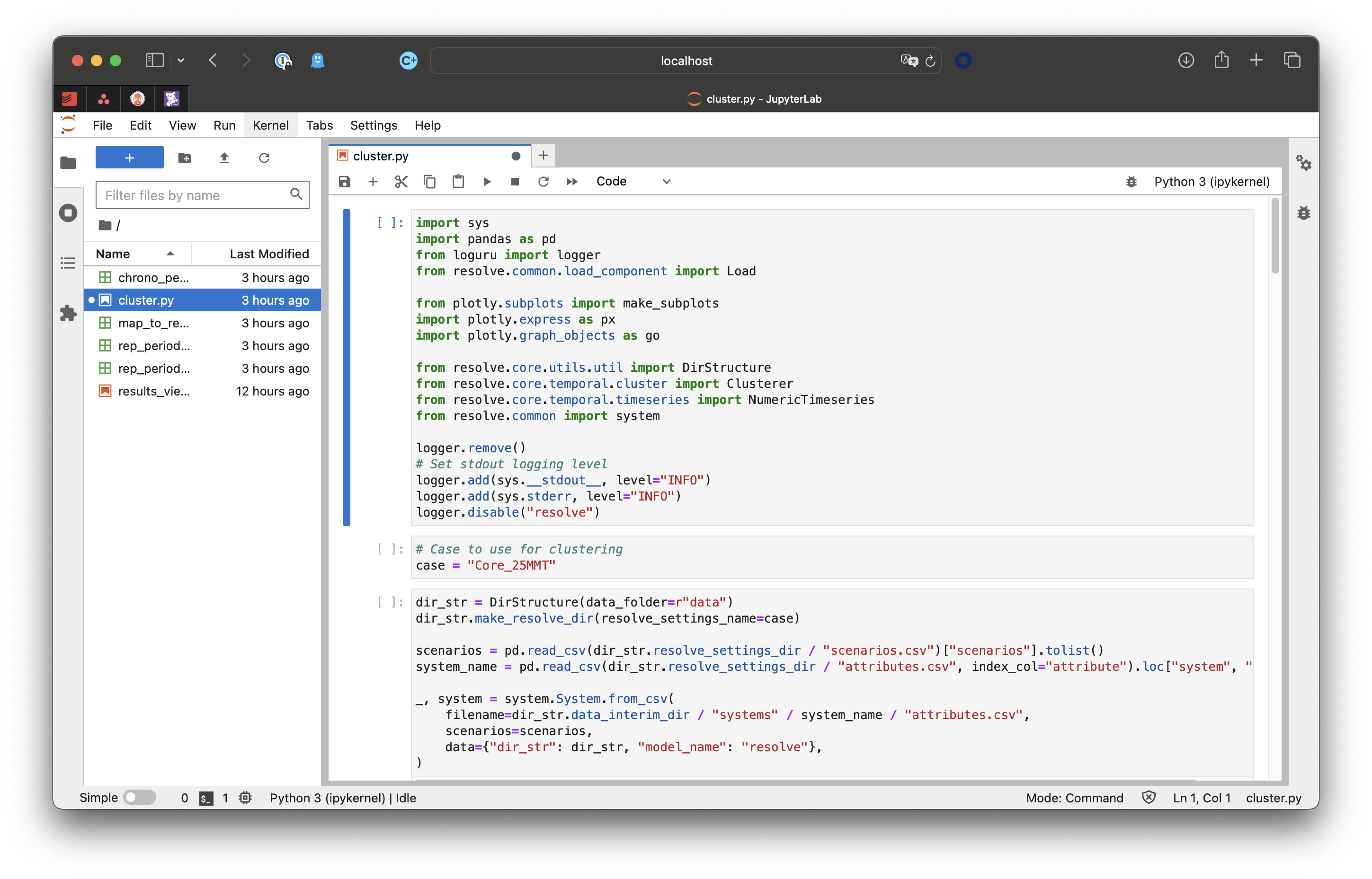
4. In the second “cell”, change the case name from “Core_25MMT” to the case you want to use. The notebook will then load the case and its corresponding system data to start the timeseries sampling process.

5. Run the cells (using the button or by using Shift + Enter keyboard shortcut). (For Jupyter notebook basics, users can start here).

6. If the notebook runs successfully, a CSV file will be created in the ./notebooks folder called map_to_rep_periods.csv. Paste the data in that CSV into the “Rep Periods” tab of the Scenario Tool (insert columns in the yellow input table areas as-needed).

7. Toggle between different timeseries samples by updating your case settings on the “Case List” tab.