🏃‍♀️ Toy Model: How-tos and Homeworks

Sept 11, 2024

60 min read

Quick Start Guide

In this section, we will provide a high-level guidance of the Recap workflow that users should go through to set up and run different kinds of Recap cases.

💻 Navigate the UI

The toy/template UI that will be used for all examples is: “./Recap-Resolve Scenario Tool.xlsm”.
This UI is pre-populated with data for a toy ISO New England system.

🏃 Example 1: Run a Single Recap Run

💭 the takeaway: here you will learn how to run a simple base case in Recap and then check the reliability of the toy system in the short term, e.g., 2030.

1. Define and save System: In the “ System” tab, define all the Components of the system (pre-populated in the example UI), then click on the “1. Save System Configuration” button to save it. You will need to assign a name in row 4 to this user-defined system before saving.

What’s happening here?

What’s happening here?

This macro will record the entries in this tab in a specific format, create necessary CSV files for executing the model, and save them in the project folder.

Those System inputs are saved here: “./data/interim/systems/[YourAssignedSystemName]”.

2. Define and save Components: Each worksheet after the “Components →” tab defines elements of a potential system. Set up respective elements of the component (pre-populated in the example UI) in each worksheet and then click VBA button “2. Save Component Data for Model” in the “Components →” tab to set up components. Model Name should be set to Recap as well.

What’s happening here?

What’s happening here?

This macro will read and re-format the data in each worksheet, then save them as csv files in the project folder.

You shall see each tab saved as a folder here: “./data/interim/”.
You shall also see Linkages between components created in “./data/interim/linkages”.

3. Create your Case: Navigate to “Recap Case Settings” tab and fill in calculation settings of the case to run (pre-populated in the example UI). This run is aiming at calculating system reliability w/o tuning, so flip “calculate_reliability” to be TRUE. No need to modify other input settings. You can then assign a “Case Name”, e.g. “Base_Case_run”, and press “Save Case Settings” button to save your defined case.

What’s happening here?

What’s happening here?

All case settings are stored under the folder “./data/settings/Recap”. Each time a case is created, a sub-folder will the case name will be created in the master Recap folder.

You shall track case-specific calculation settings saved in each sub-folder.

4. Refresh the case list: Now in the “Case Dashboard” tab, click VBA button “Update List of Saved Cases” to refresh the full list of saved cases from the “Recap Case Settings” tab. This allows you to see which cases are available.
   
   
   

5. Choose the case and execute the model: Click the cell that contains the correct case and press “Run Recap Cases” button to run the selected case. This will initiate a separate Command Prompt window showing the progress of the model.

can I execute the model from the command line?What’s happening here?

can I execute the model from the command line?

Recap 3.0 can also be run from the command line! This can be useful if the UI macros are giving you trouble.

To run Recap from a command line, open a Command Prompt (or another terminal app, like PowerShell) in the “./kit/Recap/” folder and activate the environment using the following command: conda activate [environment-name] (per the setup example above: conda activate nve-Recap-kit). Then use the following command to run the case: python run_model.py.

To specify which case you’re running, update the cases_to_run.csv within the “./data/settings/Recap/” folder. Users now only have the choice to run one single case, the developer team is working on speeding modeling up to run a batch of cases in parallel.

6. View results: For this test case, you should expect the model to finish in about 2 minutes. After the case is completed, navigate to "/reports/Recap/" folder and find the right sub-folder for the case you just ran. Within the case folder, check out system reliability metrics in the “reliability_results.csv” file. The LOLE result should be roughly 19.01/yr.
   
   
   

🏃 Example 2: Run a Marginal ELCC Case

🏃 Example 2: Run a Marginal ELCC Case

💭 the takeaway: here you will learn how to calculate a resource’s marginal ELCC in Recap

1. Determine the base case: Make sure you have a base case defined & have respective System and Components created. This will be the base case portfolio relative to which the ELCC cases become marginal. If you’re starting from a blank UI, set up the base case following the procedure in Example 1.
   
   
   

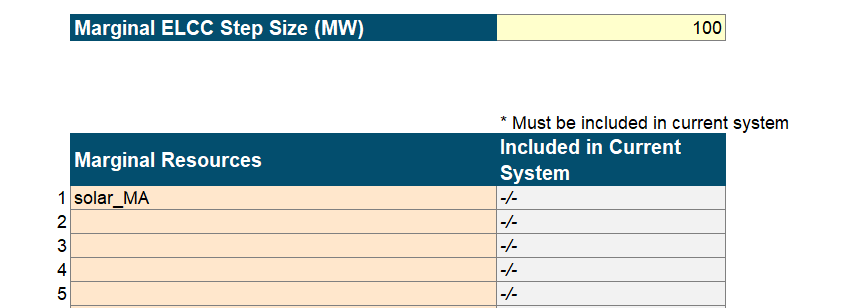
2. Select the resource and decide step size: Pick one existing resource in the portfolio, then add it into the “Marginal Resources” table in the “Recap Case Settings” tab. In the “Marginal ELCC Step Size (MW)” cell above, define the incremental capacity added to the resource relative to base case. In this guiding example, calculate marginal ELCC for additional 100 MW tranche of “solar_MA”.

3. Save the new case and execute the model: To use the marginal ELCC functionality in Recap 3.0, flip “calculate_marginal_ELCC” to TRUE in the Recap Case Settings table. Since ELCC is calculated as the difference of capacity short / deficit between the base case and marginal case, you also need to flip “calculate_perfect_capacity_shortfall” to TRUE to initiate the calculation of base case capacity short. Next, assign a name and save the new case by pressing “Save Case Settings” VBA button, then follow step 4 & step 5 in Example 1 to write and run the case.

Note on saving a new case

Note

Note that saving a new case involves no system components or linkages updates. At any time the user wishes to define new components or modify attributes of a specific component, it is required to click “1. Save System Configuration” and “2. Save Component Data for Model” button again.

Note on saving a new case

What’s happening here?

Upon saving the case, you shall see a new sub-folder created here with the case settings: “./data/settings/Recap/custom_ELCC_surface.csv”.
It is important for user to confirm that these calculation settings are set appropriately for specific use-case, so it is recommended for user to compare this sub-folder with that of the base case (from Example 1) to see how case settings have changed in a marginal ELCC case run.

You shall find the two differences exist in “./ELCC_surfaces/marginal_ELCC.csv” and “./case_settings.csv”.

4. View results: For this test ELCC case, you should expect the model to finish in about 5 minutes. After the case is completed, navigate to "./reports/Recap/" folder and find the right sub-folder for the marginal ELCC case. Within the case folder, check out marginal ELCC result for “solar_MA” in the “ELCC_results.csv” file. The ELCC should be roughly 53 MW.

Note

Note that ELCC can be found IN the result csv file (column incremental_ELCC), which is the difference in capacity shortfall/surplus of the base case (column base_case_perfect_capacity_shortfall) and marginal case (column perfect_capacity_shortfall).

🏃 Example 3: Run an ELCC Surface Case

🏃 Example 3: Run an ELCC Surface Case

1. Determine the base portfolio: Make sure you have a base portfolio defined & have respective System and Components created. This will be the base relative to which the ELCC surface become marginal. If you’re starting from a blank UI, set up the base case following the procedure in Example 1.

Note

Any ELCC curve or surface must use a resource, or set of resources, included in the system. If you want to use a new resource, first define it in the system with 0 capacity as an initial input.

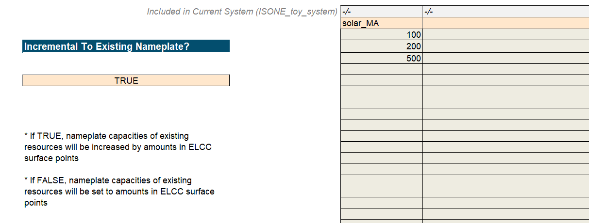
2. Define the ELCC surface: Scroll down to the bottom of “Recap Case Settings” tab to define ELCC surfaces. Select the resource that constitute the ELCC curve (2-D) or surface (3-D), and then put the resource name in row 107. In this example, we will use the same resource and create a 2-D ELCC curve for “solar_MA” (see table below). Decide the penetration level at each surface point and then flip “Incremental To Existing Nameplate?” to be TRUE.

3. Save the new case and execute the model: To use the ELCC Surface functionality in Recap 3.0, flip “calculate_ELCC_surface” to TRUE in the “Recap case Settings” table. Save the new case by pressing “Save Case Settings” VBA button, then follow step 4 & step 5 in Example 1 to write and run the case.

What’s happening here?

What’s happening here?

Upon saving the case, you shall see a new sub-folder created here with the case settings: “./data/settings/Recap/[YourAssignedElccSurfaceCaseName]”.
It is also recommended for user to compare this sub-folder with that of the base case ( from Example 1). Similar to the marginal ELCC case, you shall find two differences exist in “./ELCC_surfaces/” folder and “./case_settings.csv”.

4. View results: For this test ELCC surface case, you should expect the model to finish in approx. 6 minutes. After the case is completed, navigate to "./reports/Recap/" folder and find the right sub-folder for the ELCC surface case. Within the case folder, check out ELCC results for tranches of “solar_MA” resource. The file should be named as the "custom_elcc_surface_ELCC_results.csv”.