Clustering
To maintain computational tractability in multi-year capacity expansion like Resolve, we often need to sample the timeseries data we’re using.
Resolve projects prior to 2018 used an in-house quadratic optimization that minimized the squared error between the overall distribution of data (binned into an arbitrary number of bins, think of a histogram) and the sampled distribution for the selected days.
From 2018-2021, Resolve projects used a slightly updated sampling methodology that switched to a multi-objective, mixed-integer linear program (MILP) that minimized the absolute distributional error. This methodo allowed users to more directly steer the optimization, including (a) specifying a specific number of sampled days and (b) force in specific days to be selected.
In both cases, since the method was sampling based on the distributional statistics, this was a “lossy” sampling method that meant that there was no easy-to-ascertain mapping between the original timeseries/calendar dates and the sampled days.
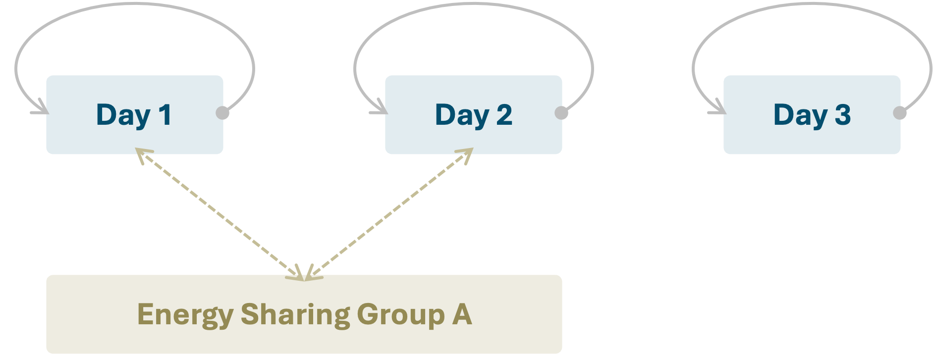
Once we had those sampled days, Resolve used an “Ourobouros”-style formulation to “wrap around” hourly linking constraints from the last hour of a day to the first. As an optional feature, energy could be “shared” between sampled days by grouping days together, as visualized in the figure below:
With the development of kit, we migrated from “old-style” temporal representation to a
“new-style” representation based on Kotzur, et al.. This move was
made (a) to reduce reliance on in-house/black-box methods and (b) to allow us to preserve chronological information
between sampled days. We are using a class of clustering methods called “k-medoid” clustering, which returns a
representative or “exemplar” from the original dataset and a mapping of all the nearest data points, which allows us to
reconstruct a “low-resolution” version of an 8760.
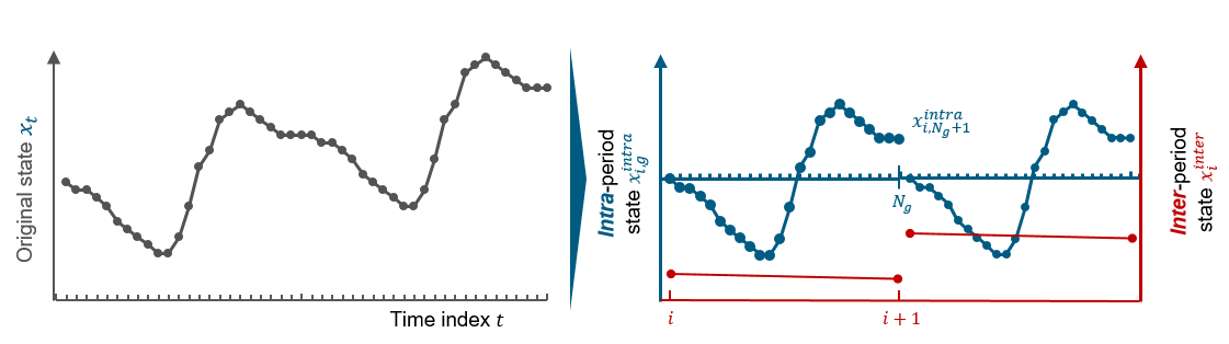
Separation of the original state into two states on two different time layers. These layers are here referred to as the
“intra-period” and “inter-period” layers, or alternately “representative” and “chronological” periods in kit.
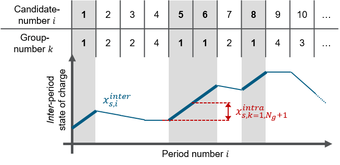
Sketched high layer inter-period state \(x^{\text{inter}}_{i}\) based on the sequence of appearance of the representative periods k. This is highlighted for period or group number 1.